Building a V-JEPA-style world model to learn driving dynamics from nuScenes
I implemented a V-JEPA-style latent-prediction world model from scratch (context and target encoders with an EMA teacher, a clip-level predictor, aggressive tube masking), trained it and an MAE pixel baseline with 2-GPU DDP, and probed both for ego-speed. With a parameter-free k-NN probe, JEPA's frozen features read speed (R² about 0.75) and clearly beat the pixel baseline, which keys on appearance: the latent-versus-pixel result the project set out to test. A high-dimensional linear probe overfit the tiny dataset and hid it, a reminder that probe choice matters at small N.
I wanted to implement a V-JEPA-style world model from scratch and find out whether it learns anything useful on driving video. V-JEPA rests on one clean idea: instead of training a video model to reconstruct pixels, you train it to predict its own latent representations of the parts it cannot see. Pixel reconstruction spends most of its capacity on detail that barely matters (exact textures, lighting, the grain of the tarmac), whereas predicting in latent space only asks the model to get the semantic content of the hidden region right. The hope is a representation that captures dynamics rather than appearance.
To test that, I picked the cleanest probe I could think of: read the ego-vehicle’s speed off the frozen encoder with a single linear layer. Speed is a continuous scalar the model is never trained to predict, so if the encoder has learned anything about motion, a linear head should recover it for free. It is a stricter test than reconstruction, which would flatter the pixel baseline by construction. So I built two models that differ in exactly one thing, the prediction target, and compared them under an identical budget.
The short answer up front:
On nuScenes-mini (10 scenes), a parameter-free k-NN probe reads ego-speed off JEPA’s frozen features (R² about 0.75) while the pixel baseline cannot (negative for every k): JEPA’s representation is organized by motion, the pixel baseline’s by appearance, which is exactly the latent-versus-pixel distinction the project set out to test. A high-dimensional linear probe overfit the roughly 40 clips and hid this at first. The result is small-scale and noisy, but it points the way the hypothesis predicted.
What follows is the build, how I kept the comparison fair, what the numbers say, and why I read them the way I do.
The idea, and the two models
A JEPA has three parts. A context encoder sees a heavily masked clip, only about 12% of the patches. A target encoder, which is an exponential moving average of the context encoder, sees the whole clip. A small predictor then tries to predict the target encoder’s embeddings of the masked patches from the context. The loss is in representation space (smooth-L1), computed only on the masked positions. Nothing is ever reconstructed in pixels.
The comparison arm is an MAE-style pixel baseline: the same ViT-B/16 encoder, but the predictor and EMA target are replaced by a small convolutional decoder that reconstructs the raw pixels of the masked patches, with an MSE loss. There is no EMA, because when the target is the raw image there is nothing for a teacher to produce. Keeping the encoder architecture identical is what makes the downstream probe a fair test: the only thing that differs between the two is what the encoder was asked to predict, latents or pixels.
The architecture, and where I simplified
A few design choices are load-bearing, and a couple are simplifications worth stating plainly.
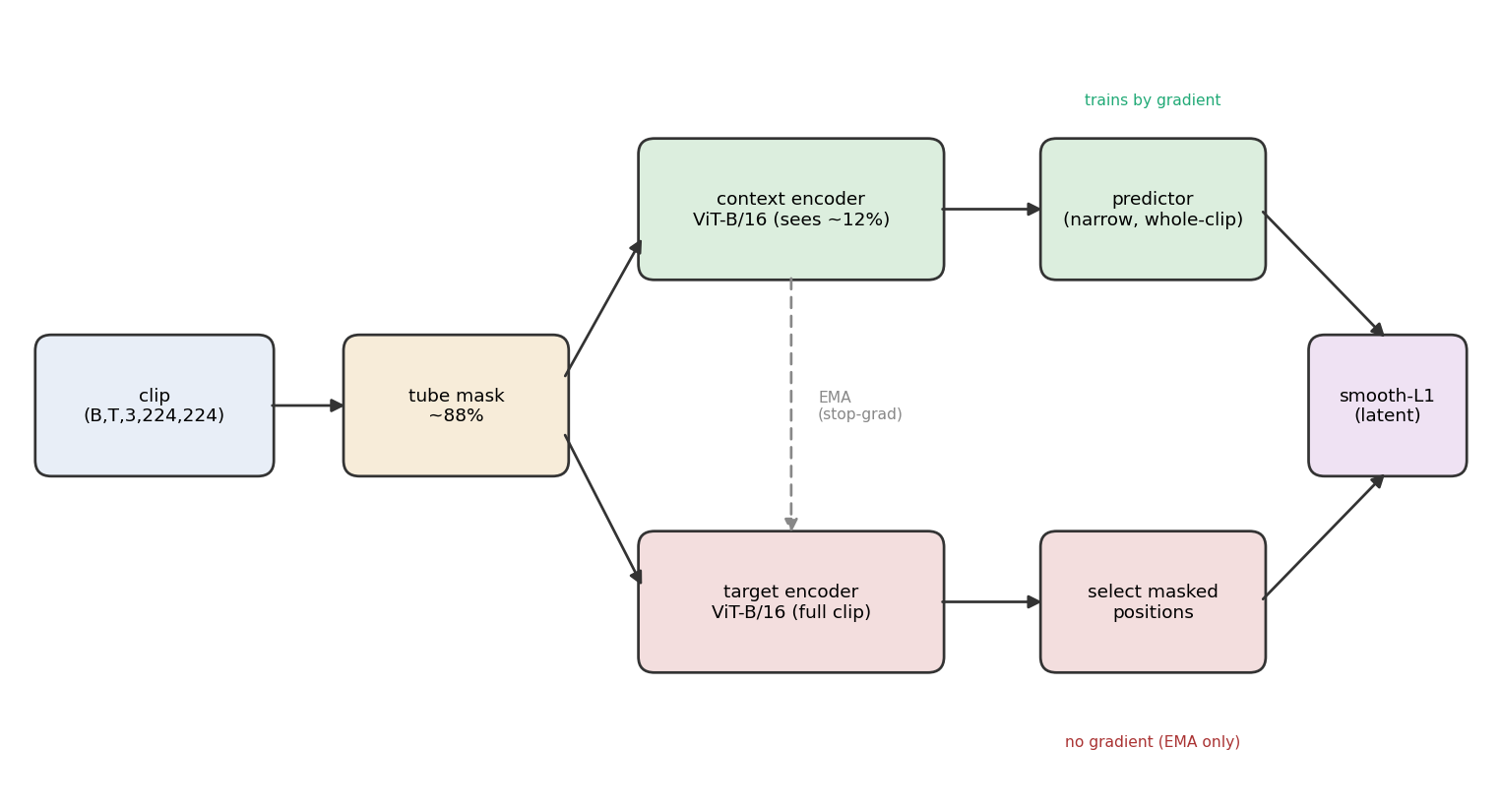
The context encoder (green) trains by gradient and sees only the visible ~12%. The target encoder (red) is an EMA copy with a stop-gradient that sees the whole clip and never enters the optimizer. The predictor models time over the whole clip, and the loss is smooth-L1 in latent space on the masked positions. The pixel baseline replaces the predictor and EMA target with a conv decoder and an MSE loss in pixel space.
The two encoders mask in opposite places. The context encoder masks its input: masked tokens are dropped before the transformer blocks, so the encoder genuinely never sees them. I verified this with a leak test, corrupting the pixels of the masked patches to garbage and confirming the context encoder’s output stays bit-for-bit identical. If it did not, the targets would leak in through self-attention and the task would collapse to copying. The target encoder masks its output instead: it encodes the full clip and we select the masked positions afterward, so the targets are context-informed.
Tube masking and bidirectional attention form an interlock. The same spatial mask is applied to every frame (a tube). This matters because the predictor uses full, bidirectional attention over the whole clip, and that would be trivial under per-frame masks, since a masked patch could just be copied from an adjacent frame where it happens to be visible. The tube removes that shortcut, because a masked position is hidden in every frame, and that is exactly what lets the predictor attend across time honestly: it has to infer the hidden region from motion in the visible patches rather than copy it. The two choices only work together.
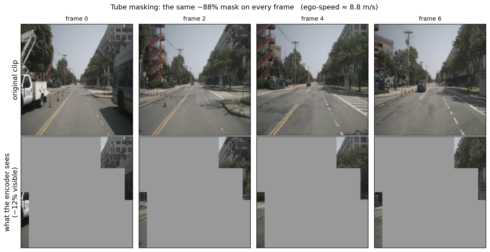
Top: the original clip. Bottom: what the context encoder actually sees, the same ~88% spatial mask on every frame, only about 12% of the patches visible. Because the scene slides under a fixed mask, no masked patch can be recovered by copying it from a neighbouring frame.
The predictor is where time lives. I use a per-frame ViT for the encoder, so the encoder itself has no temporal attention. All temporal modelling happens in the predictor, which runs over the whole clip as one token sequence with spatial and temporal positional embeddings. That is the difference between a world model and eight independent image models.
Collapse avoidance comes from the EMA target plus a stop-gradient: the loss only ever pulls the student toward a slow-moving teacher, never the other way, so the trivial solution where everything maps to a constant is not reachable. This is the BYOL/DINO/ I-JEPA trick, and I checked the wiring directly with a single-batch overfit that drops without crashing to zero, plus the target excluded from the optimizer and moved only by EMA.
Two caveats. Real V-JEPA tokenizes the clip into spatiotemporal tubelets and runs one ViT over everything, whereas my per-frame ViT plus temporal masking is a deliberate simplification, so I call it V-JEPA-style rather than a reproduction. And this is a masked representation learner, not a causal forecasting model: it does not predict the future from the past and is not rolled out, so the “world model” label is aspirational.
Training
Both models are ViT-B/16 encoders, trained with PyTorch DDP across 2 GPUs (torchrun, bf16, gradient clipping, rank-0 logging and checkpointing). The data is nuScenes-mini: 10 front-camera scenes, split by scene into 8 train and 2 val (a clip-level split would leak near-identical neighbouring frames across the split and inflate the probe). Using the roughly 12 Hz camera sweeps rather than only the 2 Hz keyframes, which is the single biggest data lever available, still yields only about 74 training clips. That is a small dataset, and as the probe will show, at this size how you read the features matters as much as what they contain.
Results
After training, I freeze each encoder and read ego-speed off it with a probe fit on the train scenes and evaluated on the held-out val scenes. I use the keyframe clips here (the canonical 2 Hz frames), which gives 39 train and 10 val clips, and pool each clip into a 6144-dim feature (8 frames times 768 dims, keeping the temporal axis since speed is temporal).
The obvious probe, a ridge linear regression, is inconclusive. Ridge is linear regression with an L2 penalty of strength λ that shrinks the weights, so a large λ pulls the predictions toward the mean. With 6144 features and only about 40 clips a plain linear fit overfits wildly, and even sweeping λ the best R² stays at or below zero for both encoders (JEPA peaks at -0.13, the pixel baseline at -0.47, where R²=0 is the predict-the-mean baseline). At face value that reads as no signal, but with this many features and so few clips it mostly reflects the probe overfitting, not the representation.
So I switch to a probe that cannot overfit: parameter-free k-NN. For each val clip, predict its speed as the mean speed of its nearest neighbours in feature space, with no weights to fit. This is a standard self-supervised eval, and it tells a completely different story:
| probe | JEPA R² | Pixel R² |
|---|---|---|
| ridge linear (best λ) | -0.13 | -0.47 |
| k-NN (k=5) | +0.75 | -2.94 |
JEPA’s frozen features read ego-speed well (R² 0.75, RMSE 2.2 m/s) and the pixel baseline cannot (R² -2.94). The gap is robust: JEPA is positive for every k I tried (1, 3, 5, 10) and the pixel baseline negative for every one.
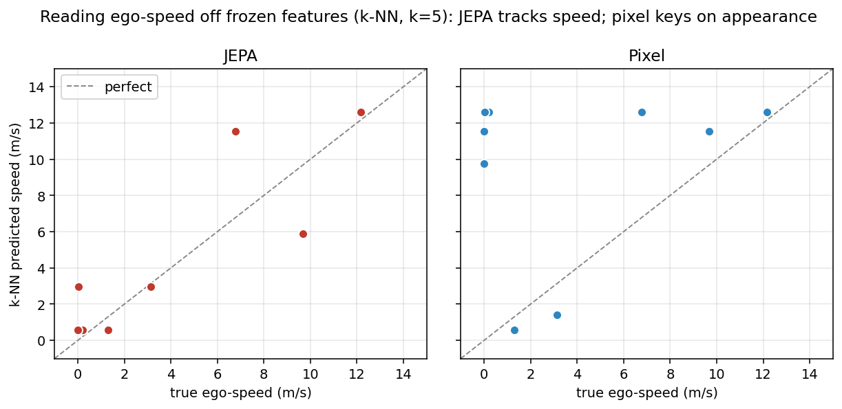
Predicted versus true ego-speed, k-NN on frozen features, held-out scenes. JEPA’s predictions track the diagonal: stationary clips come out near zero, fast clips fast. The pixel baseline puts the stationary clips up at 10 to 12 m/s, because their nearest neighbours are visually similar but fast clips from other scenes.
The predictions make the difference concrete. The val set has several stationary clips (true speed near zero). JEPA predicts them near zero and the fast clips fast. The pixel baseline predicts the stationary clips as fast, because in pixel-feature space a stopped scene looks like some moving scene that happens to resemble it. JEPA’s features are organized by motion, the pixel baseline’s by appearance. That is exactly the latent-versus-pixel distinction the project set out to test, and it is why ridge missed it: the signal lives in how the features cluster, which k-NN reads directly but a high-dimensional linear fit drowns in overfitting.
A label-free look at the features agrees. Both encoders are low-rank, with a participation ratio of about 1.2 out of 768 dimensions, so most of the variance sits in a single direction, which is what you expect from a ViT trained from scratch on so little data. The difference is what that dominant direction encodes: for JEPA it tracks speed, for the pixel baseline it tracks appearance.
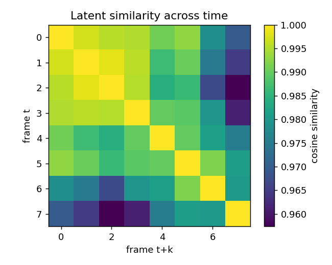
Cosine similarity between the JEPA encoder’s embedding of frame t and frame t+k. The bright diagonal is self-similarity, decaying gently off-diagonal, the shape you would want from a world model.
One caution in the other direction: more training hurt. Trained to 1000 epochs instead of 100, the ridge probe got markedly worse, and the training loss dives toward zero early then drifts back up, the signature of the objective overfitting the pretext task on so few scenes. The 100-epoch checkpoint is effectively an early-stop sweet spot, and it is what I report above.
Limitations
The evaluation is small: 39 train and 10 val clips from 10 scenes, so the k-NN R² (which ranges from 0.28 to 0.75 across k) is encouraging but noisy, and I would not over-read the exact number. The high-dimensional ridge probe overfits at this size, which is why k-NN is the more trustworthy read here, though it is also a reminder that with more data a plain linear probe should work too. Training is short and single-seed, and training longer degrades the model. And the architecture is a deliberate simplification of V-JEPA (a per-frame ViT plus temporal masking rather than spatiotemporal tubelets), so this is V-JEPA-style, not a reproduction.
Future work
In rough priority:
- More data. Full nuScenes (about 700 training scenes) rather than the 10-scene mini, which would tighten the noisy estimates and let a plain linear probe work, not just k-NN.
- Tighter error bars. The k-NN R² is estimated on 10 val clips; more validation data or cross-validation would say how solid the 0.75 really is.
- Multiple seeds, since at this size a single run leaves room for luck.
- A more faithful architecture, with spatiotemporal tubelets and a single ViT over the clip, which is both closer to V-JEPA and a stronger model.
Conclusion
I set out to implement a V-JEPA-style world model and test whether latent prediction yields a more speed-legible representation than pixel prediction. It does. With a probe robust to the small dataset, a parameter-free k-NN, JEPA’s frozen features read ego-speed (R² about 0.75) and clearly beat the pixel baseline, whose features key on appearance rather than motion, which is the outcome the hypothesis predicted. The implementation is verified end to end: a leak-tested context encoder that provably never sees the targets, anti-collapse wiring checked with a single-batch overfit, correct EMA semantics, and training under 2-GPU DDP. Two honest qualifications. The high-dimensional ridge probe overfit about 40 clips and at first hid the result, a reminder that at small sample sizes the probe can dominate the conclusion. And the evaluation is small (10 val clips, single seed, and training longer degrades the model), so the headline number is encouraging rather than airtight, and the fix for both is more data. But the core finding holds in the direction the project was built to test: predicting latents, not pixels, gave the representation that actually knows how fast the car is going.
Code: github.com/JamesSteiner/jepa-world-model
References
- Assran et al. (2023), Self-Supervised Learning from Images with a Joint-Embedding Predictive Architecture (I-JEPA), arXiv:2301.08243.
- Bardes et al. (2024), Revisiting Feature Prediction for Learning Visual Representations from Video (V-JEPA), arXiv:2404.08471.
- Grill et al. (2020), Bootstrap Your Own Latent (BYOL), arXiv:2006.07733.
- He et al. (2021), Masked Autoencoders Are Scalable Vision Learners (MAE), arXiv:2111.06377.
- Caesar et al. (2020), nuScenes: A Multimodal Dataset for Autonomous Driving, arXiv:1903.11027.