Flow vs. regression vs. diffusion: a controlled comparison of VLA action heads
I trained the same VLA action expert three ways (flow matching, L1 regression, and DDPM diffusion) and changed nothing else, to see how much the objective actually matters.
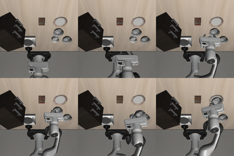
Modern Vision-Language-Action (VLA) models almost all share a recipe: a big pretrained vision-language backbone, plus a small action head that turns its features into the actual motor commands. Teams disagree about what that head should be, some use diffusion (Diffusion Policy, Octo), some flow matching (π0, SmolVLA), some plain regression, and each choice comes with a story about why it’s better. I wanted to know how much the choice actually matters, so I ran the experiment that isolates it: hold everything else fixed and vary only the action objective. Same backbone, same conditioning, same expert network, same data, same training recipe, only the loss and the sampling procedure change.
The short answer, on LIBERO-Spatial:
Deterministic L1 regression matches flow matching (~70–74% success) at half the inference cost, and both beat DDPM diffusion (39%), even when diffusion is given twice the training budget. The iterative samplers bought no accuracy here.
In what follows I unpack each objective, how I kept the comparison fair, what the numbers say, and the work it took to trust them.
The base model: SmolVLA
I built on SmolVLA, a compact, open VLA from the LeRobot project. It has two parts:
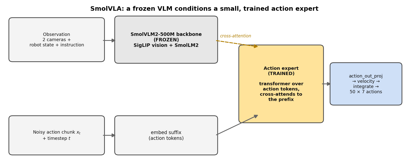
A frozen vision-language backbone SmolVLM2-500M, a SigLIP vision encoder plus a SmolLM2 language model, ingests the two camera views, the robot’s proprioceptive state, and the instruction, and turns them into a sequence of conditioning tokens called the prefix. A small, trained action expert (~100M parameters), a separate transformer, then produces the action chunk. Crucially it doesn’t read a pooled summary of the prefix; its layers cross-attend to the backbone’s representation, so every predicted action is grounded in the scene and the instruction.
SmolVLA predicts a chunk of ~50 future actions at once, which the robot executes before re-planning. Predicting a whole chunk rather than one action at a time is a standard move (action chunking): committing to a short open-loop plan curbs the compounding error a single-step policy accumulates as each prediction feeds the next observation, and it keeps the executed motion temporally consistent. Its native head is flow matching but the expert is ultimately just a transformer mapping (action tokens, prefix) → output, and nothing stops me from training that same expert with a different objective. That modularity is what makes the controlled comparison possible: freeze the backbone, keep the expert architecture fixed, and change only what the expert is trained to output.
The three objectives
All three are trained by imitation learning (behavioral cloning): the data is a set of teleoperated demonstrations, and each objective trains the expert to reproduce the action the demonstrator took in a given state. They take the same input, a contextualized summary of the cameras, robot state, and instruction, and produce the same output, a chunk of the next ~50 actions scored against the demonstrated one. They differ only in how they parametrize and train that prediction.
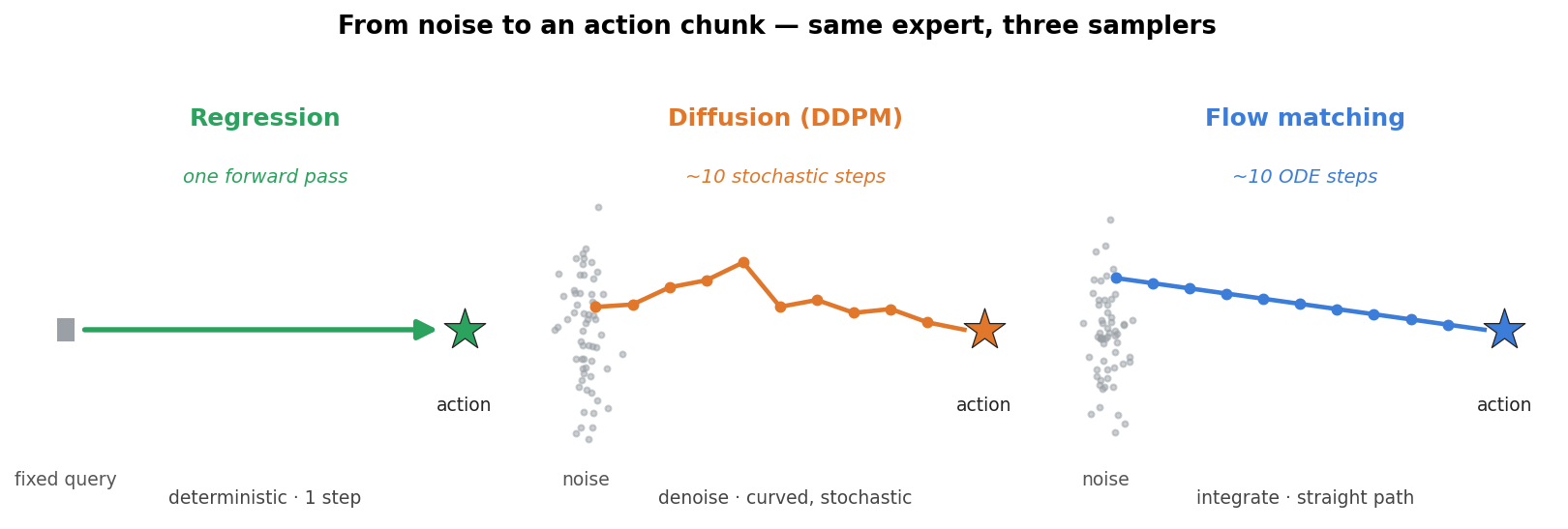
Regression is the obvious baseline: run the network once, directly output the action chunk, and train it to match the demonstration with an L1 loss. One forward pass, no randomness, no iteration. This is the “do we even need a generative head?” control.
Diffusion (DDPM) models the distribution of actions by learning to reverse a gradual noising
process. The forward process takes a demonstrated action chunk a and mixes in Gaussian noise on a
schedule indexed by a timestep t,
where the noise level grows with t. The network is trained to undo this, predicting the noise that
was added under a plain regression loss,
Generation starts from pure noise and denoises step by step back to a clean action, each step using
the predicted ε to peel off a little noise. I sample with DDIM, a deterministic sampler that
needs only ~10 steps instead of the full chain. The appeal is that diffusion can represent multimodal
action distributions, several valid ways to do a task, at the cost of many forward passes per action.
Flow matching is a continuous-time cousin of diffusion, and it’s SmolVLA’s native head. Instead of a stochastic schedule it lays down a straight-line path between noise and the action,
\[x_t = t\,\varepsilon + (1-t)\,a, \qquad t \in [0, 1],\]so t = 1 is pure noise and t = 0 is the action. Differentiating, the path moves at a constant
velocity,
and the network is trained to predict that velocity,
\[\mathcal{L}_{\text{flow}} = \mathbb{E}_{t}\,\big\lVert\, v_\theta(x_t, t, \text{context}) - (\varepsilon - a) \,\big\rVert^2 .\]Generation starts at noise and integrates the learned velocity field, an ODE, from t = 1 down to
t = 0. Because the target path is straight, a few large Euler steps approximate it well, which is why
flow tends to need fewer steps and behave more stably than diffusion’s curved, stochastic trajectories.
Seen side by side, diffusion and flow are the same idea with different geometry: both sample a noise
level, regress a fixed vector target (the added noise ε for diffusion, the velocity ε − a for flow)
under an MSE loss, and at inference walk from noise to action over a handful of steps. Regression is
the stripped-down case, no noise and no iteration, predicting the action in one shot. The three thus
span a range from a single deterministic forward pass to full distribution modeling, and the question
is whether that extra machinery actually helps a policy act.
Isolating the objective
The trap in comparisons like this is an architecture confound. Different objectives are usually built with different networks, a small MLP for regression, a large transformer for diffusion, so when their success rates differ the cause is ambiguous: it could be the objective, or it could simply be that one network had more capacity than the other. The two are entangled, and no single comparison can separate them.
So I forced all three to share the exact same SmolVLA ~100M-parameter action expert, the transformer that cross-attends to the frozen backbone’s features:
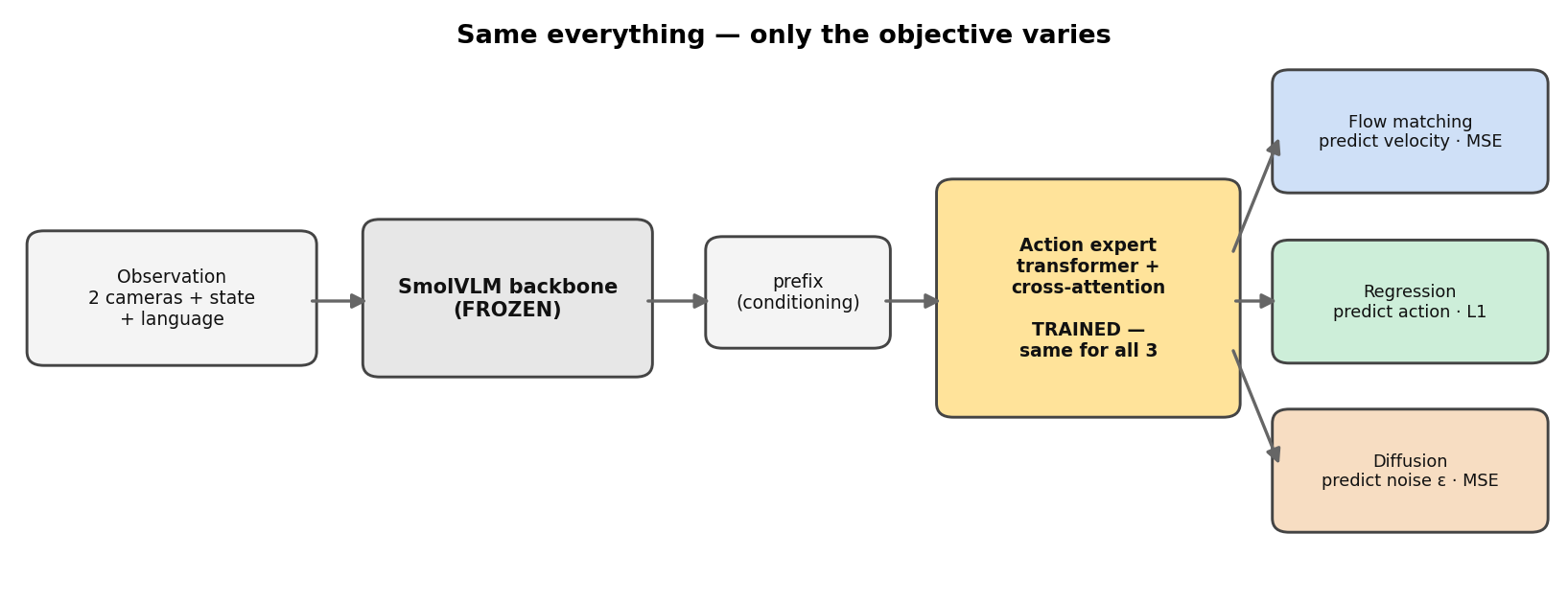
The SmolVLM backbone stays frozen, so the conditioning is identical for everyone, and the action expert is the only thing trained with the same optimizer and learning-rate schedule across all three runs. Only the loss and the sampler change: flow uses the native flow-matching loss, regression feeds the expert a fixed query and an L1 loss, and diffusion feeds it noised actions and trains it to predict ε. Any gap in the results is then attributable to the objective, full stop.
I trained each head on the lerobot/libero dataset (backbone frozen, expert fine-tuned) and evaluated
by running the policy closed-loop in the LIBERO simulator which executes its actions and
checks task success, the same way it would be deployed.
Results
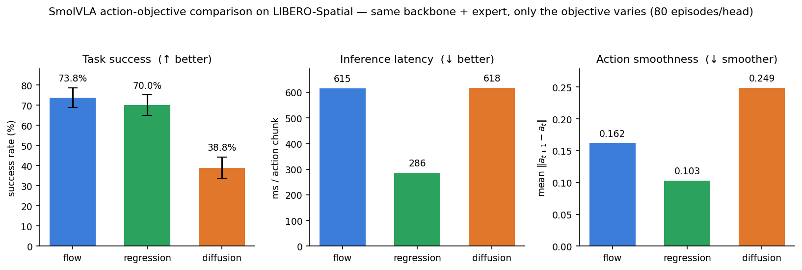
10 tasks × 8 rollouts = 80 episodes per head, reporting success (with a binomial standard error), inference latency, and action smoothness:
| objective | success ± SE | inference latency | action smoothness ↓ | train steps |
|---|---|---|---|---|
| flow matching | 73.8% ± 4.9 (59/80) | 615 ms / chunk | 0.162 | 30k |
| L1 regression | 70.0% ± 5.1 (56/80) | 286 ms / chunk | 0.103 | 30k |
| DDPM diffusion | 38.8% ± 5.4 (31/80) | 618 ms / chunk | 0.249 | 60k |
Latency and smoothness were measured on Apple-Silicon MPS, so read the latency as a ratio of one forward pass vs. ten denoising steps rather than an absolute; the numbers shift on other hardware, the ordering does not.
Three things stand out:
- Flow ≈ regression. The 3.8-point gap sits well inside the combined standard error (~7), so flow’s apparent edge isn’t significant.
- Both decisively beat diffusion. The 31–35-point gaps are ≈4–5 standard errors, and diffusion needed twice the training budget even to reach 39%: at the matched 30k it managed just 7%. The ε-objective was the least sample-efficient of the three here.
- Regression is the practical winner. It ties flow on success while running 2× faster (one forward pass vs. ten denoising steps) and producing the smoothest trajectories. For this head, iterative sampling buys no accuracy, and diffusion costs both speed and smoothness.
It’s a counterintuitive result: the simplest objective gives the best trade-off here, and the most elaborate sampler fares worst.
Validating the evaluation
In addition to setting up the heads; getting numbers worth trusting was a big part of the work in this project.
The expert trains with the standard warmup-then-cosine learning-rate decay. (An early run that held the rate constant trained to a clean loss but failed every rollout, a useful reminder that a falling loss and a working policy are different claims, and only a closed-loop rollout tells them apart.)
Before trusting any success number, I checked that the evaluator was correct, not just the model. A public LIBERO checkpoint scores ~58% through the same harness, and ground-truth demonstration actions replayed from the matching simulator state solve the task. With the measurement pinned down, a 0% means the model, not the meter.
Episode count mattered more than I expected. At 30 episodes per head the ranking was wrong: regression and diffusion looked tied around 57%, with flow ahead. Pushing to 80 episodes flipped it: regression climbed to 70%, diffusion fell to 39%. The headline only means something with the uncertainty attached, and those error bars are why I trust the gaps in the table.
Interpreting the result
Why does the simplest objective do so well? The most likely explanation is that LIBERO-Spatial’s demonstrations are close to unimodal, that is for each task there is essentially one sensible way to reach and place the object, and the demonstrations broadly agree on it. When the distribution of good actions for a given observation has a single mode, predicting its mean is enough, and a deterministic regressor does exactly that. The generative heads’ headline advantage, representing several valid behaviors at once, has nothing to bite on here.
The same reasoning predicts when the ranking should flip. An L1 or L2 regressor trained on a genuinely multimodal target averages over the modes, and the average of two valid behaviors is often itself invalid: the mean of “go around the left” and “go around the right” is “drive straight into the obstacle.” On data with real multimodality, more diverse demonstrations, several operators, or tasks with several valid strategies, regression should begin to mode-average and degrade, while flow and diffusion, which model the whole distribution, hold up. The tie I measured is a property of this benchmark’s data, not a general verdict on objectives.
Diffusion’s weaker showing has a second cause beyond multimodality: within this budget it is harder to
optimize and to sample. Its target, the noise ε at every noise level, is a noisier regression
problem than flow’s single constant velocity, and with only ten DDIM steps any error in the predicted
ε compounds over the trajectory. That it needed twice the training steps just to reach 39% fits this
picture, diffusion is the most data- and compute-hungry of the three. More training, more inference
steps, or a better-tuned noise schedule would likely narrow the gap to flow, but flow’s straight-line
path is inherently friendlier to few-step sampling, so on a tight inference budget I would still expect
it to lead.
Takeaways
For this VLA head on this benchmark:
- Sophistication didn’t pay. One-shot L1 regression matched the generative heads on success while being faster and smoother.
- Flow matching ≥ diffusion, in both success and sample efficiency (flow converged in half the steps). If a generative head is needed, flow’s straight-line formulation is the better default here.
- Measure the policy, not the loss, and bring error bars.
That’s the point of a controlled comparison: it isolates the one variable everyone argues about, on a real benchmark including when the simple thing wins.
Future work
This is one head, one task suite, one seed, so the natural next steps follow from the limitations. The first is more seeds and the other LIBERO suites (Object, Goal, Long), to see whether the flow–regression tie holds. The most informative test is the multimodality prediction above: rerun the comparison on a task with several genuinely valid strategies, where regression should start to mode-average and the generative heads should pull ahead. I’d also like to push diffusion harder, more inference steps, a stronger sampler, longer training, to find where it plateaus, and to unfreeze more of the backbone rather than training only the expert. The measurement that ultimately matters is a real robot, not a simulator.
Code, trained checkpoints, and full reproduction commands: github.com/JamesSteiner/vla. Built on SmolVLA (LeRobot) and the LIBERO benchmark.